
Statistics Chapter 1 Statistics
Statistics may be defined as the science of collection, presentation, analysis, and interpretation of numerical data.
⇔ Data: Data are the collection of expressions or numbers by an individual or an institution for some purpose and are used by someone else in another context.
⇔ Variable: The changing numerical character is called a variable.
⇔ Example: Temperature in a day, and the daily expenditure of a family are variable.
Two types of variables:
- Discrete variable,
- Continuous variable
Example:
- The number of members of a family, the temperature of the day, etc. are discrete variables.
- The height and weight of students, etc. are continuous variables.
⇔ Attribute: In statistics the varying or changing quality is called an attribute.
Read and Learn More WBBSE Solutions For Class 9 Maths
⇔ Range: The difference between the highest and lowest values of a given data is called range.
Example: From data 10, 12, 20, 35, 49, 15, 22, 48 the range is 49 – 10 = 39
⇔ Frequency: The number of times an observation occurs in the given data is called the frequency of the observation.
⇔ Class or class interval: The variables having extended range can be divided into a few classes. Each of these types of classes is called a class or class interval.
⇔ Class frequency: The number of values of a class included in a class is called class frequency.
⇔ Class-limit: The two end-values of the class interval is called class-limit.
The lesser value of the class limit in a particular class interval is called lower class limit and the larger value is called the upper-class limit of that class interval.
Example: In class 15-20 the lower limit is 15 and the upper limit is 20.
⇔ Class-boundary: The gaps of the class limits of any consecutive classes of statistical data are extended to the two limits, these two limits are called class-boundaries of those classes.
The lesser value is called the Lower class boundary and the greater value is called the Upper-class boundary.
Example: For classes 10-20, 20-30, 30-40,…, in class (20-30) the lower class boundary is 20, and the upper class boundary is 30.
In this class limit and class boundary are same.
Let the difference between the upper-class limit of a class and the lower-class limit of it is next class = d
Then in class (l1 -l2) the lower class boundary is \(\left(l_1-\frac{d}{2}\right)\) and the upper class boundary is \(\left(l_2+\frac{d}{2}\right)\).
Example: The class boundaries of classes 1-10, 11-20, 21-30, ……are 0.5 – 10.5, 10.5 – 20.5, 20.5 – 30.5
⇔ Class size or class length: The difference of the two class boundaries of a class is the class- size or class length.
∴ Class-size = Upper-class boundary – Lower class boundary.
In classes 0-10, 10-20, 20-30,…….., the class size of the class (20-30) is 10.
In classes 1-10, 11-20, and 21-30, the class size of class 21-30 is (30.5- 20.5) or 10
⇔ Midpoint or mid-value or class mark: The value of the variable that lies exactly at the middle of two class boundaries is called the Mid-value or class mark of that class.
The mid value of a class-interval
= \(\frac{\text { Upper class limit }+ \text { lower class limit }}{2}\)
= \(\frac{\text { Upper class-boundary }+ \text { lower class }- \text { boundary }}{2}\)
Example: The mid value of class (20-30) is \(\frac{20+30}{2} \text { or } \frac{50}{2} \text { or } 25\)
⇔ Relative frequency: The ratio of class frequency of a class and total frequency of any classified statistical data is called the relative frequency of that class.
Relative frequency =\(\frac{\text { Class }- \text { frequency }}{\text { Total frequency }}\)
⇔ Frequency density: The ratio of class frequency and the class size of the class in any classified data is called frequency density.
Frequency density of a class = \(\frac{\text { class frequency of that class }}{\text { class }- \text { size }}\)
⇔ Percentage frequency: When relative frequency is expressed in percentages, it is called percentage frequency.
Percentage frequency of a class = \(\frac{\text { class frequency of that class }}{\text { Total frequency }} \times 100\)
⇔ Cumulative frequency distribution: The frequency of the first class is added to that of the second and this sum is added to that of the third and so on, then the frequencies so obtained are known as Cumulative frequency.
When the cumulative frequency of each class in a frequency distribution table is shown, it is called a cumulative distribution table.
⇔ Two types of cumulative frequency distribution table are constructed:
- Less than type cumulative frequency: The new frequencies were obtained by adding class frequencies successively in the above frequency distribution table.
- This type of frequency distribution table is called less than type cumulative frequency distribution table.
- More than type cumulative frequency distribution table: The new frequencies are obtained by adding class frequencies successively from the below frequency distribution table.
This type of frequency distribution table is called more than the type of cumulative frequency distribution table.

Histogram: The graphical representation of a classified frequency distribution of continuous variables is called Histogram.
Frequency polygon: A frequency polygon is the graphical representation of a frequency distribution that is expressed through the classes of equal size of a continuous variable.
Statistics Chapter 1 Statistics True Or False
Example 1. Relative frequency is determined by class frequency and class length.
Solution: Relative frequency of a class = \(=\frac{\text { frequency of that class }}{\text { total frequency }}\)
So if total frequency are not given then it is impossible so determine the relative frequency.
∴ The statement is False.
Example 2. In classes 6-10, 16-20, 26-30,……, the lower class boundary of the second class is 13
Solution: The difference between the first two class is (16 – 10) or 6
Lower class boundary of the second class is 916 – \(\frac{6}{2}\) or 13
∴ The statement is True.
Statistics Chapter 1 Statistics Fill In The Blanks
Example 1. For the construction of the histogram, the values of the ________ variable are taken along X-axis
Solution: Continuous.
[If discontinuous variables are given then firstly it is converted into a continuous class boundary]
Example 2. For the construction of a frequency polygon, the values included in a class are concentrated at the _______ of the corresponding class.
Solution: midpoint.
Statistics Chapter 1 Statistics Short Answer Type Questions
Example 1. In a continuous frequency distribution table if the mid-point of a class is m and the upper class boundary is m, then find out the lower class boundary.
Solution: Let the lower class boundary of the class is n.
The upper-class boundary is u
∴ The midpoint of that class is \(\frac{x+u}{2}\)
According to question \(\frac{x+u}{2}\) = m
⇒ n + u = 2m
⇒ x = 2m – u
∴ The lower class boundary is (2m – u)
Example 2. In a continuous frequency distribution table, if the mid-point of a class is 42 and class size is 10, then write the upper and lower limit of the class.
Solution: Let the upper limit is a and lower limit is b
∴ The mid-point is \(\frac{a+b}{2}\) and class size is (a – b)
According to question, \(\frac{a+b}{2}\) = 42
⇒ a + b = 84 ……(1)
and a – b = 10…..(2)
(1) + (2) we get, a + b + a – b = 84 + 10
⇒ 2a = 94
a = \(\frac{94}{2}\)= 47
∴ b = 84 – 47 = 37
∴ The upper and lower limit of the class are 47 and 37 respectively.
Example 3.

Find the frequency density of the first class of the above frequency distribution table.
Solution: The difference between the two consecutive class is 1
∴ The lower-class boundary and upper-class boundary of the first class are (70 – \(\frac{1}{2}\)) = 69.5 and (74 – \(\frac{1}{2}\)) = 74.5 respectively.
Class size 74.5 – 69.5 = 5
The frequency density = \(\frac{\text { frequency of the } 1 \text { st class }}{\text { class size }}=\frac{3}{5}=0.6\)
Example 4.
Find the relative frequency of the last class of the above frequency distribution table.
Solution: Relative frequency of last class = \(\frac{\text { frequency of that class }}{\text { Total frequency }}=\frac{8}{20}=0.4\)
Example 5. Write from the following examples which one indicates attribute and which one indicates variable.
- The population of the family
- Daily temperature
- Educational value
- Monthly income are not fixed.
- Grade obtained in Madhyamik Examination.
Solution:
- The population of the family are always changeable. So it is variable.
- Daily temperature is always changeable, it is a variable.
- Educational value indicate attribute.
- Monthly income are not fixed. It is a variable.
- Grade obtained in Madhyamik Examination are indicates attributes.
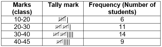
Example 6. Given below are the marks obtained by 40 students in Bengali in an Examination of School.
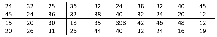
Construct a frequency distribution table for the above-given data.
Solution:
Example 7. Construct a frequency distribution table from the following cumulative frequency: distribution table, given below

Solution:

Example 8. In a frequency distribution table, the mid-value of five classes are 15, 20, 25, 30, and 35, and their corresponding frequency are 2, 4, 3, 6, and 8 respectively; prepare a frequency distribution table for the construction of the Histogram.
Solution: The difference of mean value between two consecutive class
= 20 – 15 = 25 – 20 = 30 – 25 = 35 – 30 = 5
The lower-class boundary and upper-class boundary of the first class are (15-\(\frac{5}{2}\)) or 12.5 and (15+\(\frac{5}{2}\)) or 17.5
So, the frequency distribution table are given below:

Example 9. The distribution of height (in cm) of 20 students is given below. Construct a histogram.

Solution:

Example 10. Draw the frequency polygon for the frequency distribution table given below:
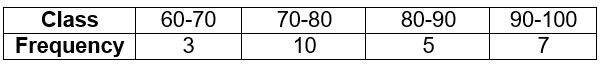
Solution: The midpoint of given classes are \(\frac{60+70}{2}, \frac{70+80}{2}, \frac{80+90}{2}, \frac{90+100}{2}\) or, 65, 75, 85, 95.
